
Graph Rewriting#
MolFoundry transforms molecules by applying rules to molecular graphs: a rule
breaks and forms bonds and relabels atoms wherever its pattern matches, following
the double-pushout (DPO) formalism from algebraic graph transformation. Rules
are written in GML and loaded with
ruleGMLString() or ruleGML().
Double pushout (DPO)#
A rule is a span of two graph morphisms
L (the left graph) is the pattern that must be found in the host graph.
R (the right graph) is what that pattern becomes.
K (the interface) is the part common to both — everything the rule matches and keeps. Whatever is in \(L \setminus K\) is deleted; whatever is in \(R \setminus K\) is created.
In GML this is exactly the three blocks of a rule [ … ]:
GML block |
Meaning |
|---|---|
|
the interface K — vertices and edges the rule preserves |
|
the part of L outside K — deleted |
|
the part of R outside K — created |
Vertices carry an id and are shared across the blocks by that id, so a context
vertex is a preserved atom that both a left (deleted) edge and a right
(created) edge can attach to.
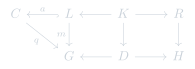
Applying the rule at a match \(m : L \to G\) into a host graph \(G\) constructs the double pushout — two pushout squares sharing the interface:
The left square removes the matched-but-deleted part \(m(L \setminus K)\), leaving
the context graph \(D\); the right square glues on the created part to produce
the result \(H\). The interface \(K\) is the glue that keeps deletion and creation
consistent — which is why an atom you mean to keep must live in context, rather
than being deleted on the left and recreated on the right.
Example#
Promoting a C–O single bond to a double bond (forming a carbonyl). Only the bond
label changes, so both atoms sit in context and only the edge moves between
left and right:
oxidize = mf.ruleGMLString('''rule [ ruleID "oxidize"
  left    [ edge [ source 0 target 1 label "-" ] ]
  context [ node [ id 0 label "C" ] node [ id 1 label "O" ] ]
  right   [ edge [ source 0 target 1 label "=" ] ]
]''', add=False)
oxidize.print()
oxidize
The depiction shows the same three graphs: L (left), K (context, center), R (right).
Nested conditions on DPO#
A plain rule fires wherever L embeds. A nested application condition narrows
that: a rule may carry one condition [ … ] block — a logical condition over the
left graph L that every match must satisfy. This is MolFoundry’s implementation
of Habel–Pennemann nested conditions, evaluated against the match before the
rewrite is performed.
A condition is built recursively:
exists [ …additions… ⟨subcondition⟩ ]— \(\exists(P \hookrightarrow P',\,c)\): the current pattern \(P\) (starting from \(L\)) extends to \(P'\) by the listed nodes and edges, and the subcondition \(c\) holds on \(P'\).not [ c ]— negation \(\lnot c\) (takes exactly one child).and [ c… ]/or [ c… ]— the connectives (any number of children).
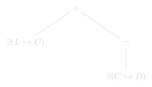
The tree above is and [ exists [ … ] not [ exists [ … ] ] ] — connectives at the
nodes, patterns growing along the branches.
The everyday case is a negative application condition (NAC),
not [ exists [ … ] ] — “this extension must not exist.” As in a rule, a
pattern lists only what it adds: vertices already visible are referred to by
id, and omitting a label means “any” (a purely structural match).
oxidize_nac = mf.ruleGMLString('''rule [ ruleID "oxidize (only if no C–H)"
  left    [ edge [ source 0 target 1 label "-" ] ]
  context [ node [ id 0 label "C" ] node [ id 1 label "O" ] ]
  right   [ edge [ source 0 target 1 label "=" ] ]
  condition [
    not [
      exists [ node [ id 100 label "H" ] edge [ source 0 target 100 label "-" ] ]
    ]
  ]
]''', add=False)
printer = mf.GraphPrinter()
printer.drawRuleConditions = True
oxidize_nac.print(printer)
oxidize (only if no C–H)
Here the pattern \(L\) (the C–O bond) may extend by an H bonded to the carbon; the NAC forbids that extension, so the rule only fires at carbons carrying no hydrogen. As a morphism the forbidden extension is:
and the condition is \(\lnot\,\exists(L \overset{a}{\hookrightarrow} C)\).
Constraint leaves#
Alongside pure pattern existence, several constraint leaves are defined as shorthands:
Leaf |
Holds when |
|---|---|
|
there is no edge between |
|
vertex |
|
the shortest-path distance between |
|
label |
OP is a comparison operator ("<", "<=", "=", ">=", ">"). The leaves nest
freely inside and / or / not and alongside exists, so an adjacency limit
and a pattern condition can be combined in one block.
Note
Shortest path constraints are NOT expressible as nested pattern conditions when OP
is ">=" or ">"! Such a combination leads to an unbounded condition expansion as we would
need to define, all shortest path patterns of size \(n, n+1, \dots, n+\infty\).
Satisfaction#
For a match \(m : L \to G\), the condition \(\exists(L \overset{a}{\hookrightarrow} C,\,c)\) holds iff there is a morphism \(q : C \to G\) with \(q \circ a = m\) — an extension of the match to the larger pattern — such that \(q\) satisfies \(c\); \(\lnot\), \(\land\), and \(\lor\) combine as usual. The rewrite is performed only at matches that satisfy the condition.
Conditions are preserved under rule composition: composing two rules always carries their conditions onto the result (there is no opt-out), so the composite fires exactly where applying the two rules in sequence would.
Composing rules#
Two rules can be composed into a single rule that represents applying them in
sequence — the DPO concurrency construction, which glues the first rule’s right
side \(R_1\) onto the second rule’s left side \(L_2\) along an overlap. MolFoundry
exposes it through RCEvaluator and four operators that
differ only in how that overlap is chosen:
Operator |
Overlap of \(R_1\) and \(L_2\) |
|---|---|
any common subgraph (the general case) |
|
all of \(L_2\) embeds into \(R_1\) |
|
all of \(R_1\) embeds into \(L_2\) |
|
empty — the disjoint juxtaposition |
rc = mf.RCEvaluator(mf.inputRules)
composites = rc.eval(first *mf.rcSuper* second)
The number of common overlaps can grow combinatorially, so
iterate() evaluates lazily: it yields the
composites eval() would return, skipping
rejected overlaps, and enumerates overlaps only as the loop asks for the next
composite. Predicates reject overlaps by their intermediate graph or the
composite’s input or output side.
def at_most_four_bonds(g):
    return all(v.degree <= 4 for v in g.vertices if v.stringLabel == "C")

expr = first *mf.rcCommon(connected=False, intermediatePredicate=at_most_four_bonds)* second
for composite in rc.iterate(expr, onlyUnique=False):
    ...
A bound like this is better stated as an
IncidenceConstraint: a condition on the edges at every
vertex with given labels, which all three graphs must satisfy. It rejects exactly
what the equivalent predicate rejects, but the engine evaluates it itself and the
common-overlap search uses it to skip every partial overlap no extension can make
valid, instead of composing each candidate and asking Python about it. Conditions
are counts of edges (IncidenceCount, optionally filtered by
edge and neighbor label and weighted by edge label) combined with
AllOf, AnyOf and
Not. Predicates still run afterwards, on the overlaps the
constraints admit.
valence = mf.IncidenceConstraint("C", "<=", 4, edgeWeights={"-": 1, "=": 2, "#": 3})
expr = first *mf.rcCommon(connected=False, constraints=[valence])* second
In the rule algebra, a rule’s jump closure is the observable that counts its
applications. dpoJumpClosure() gives I ← K → I on the
rule’s input I, including the dangling condition of every vertex the rule
deletes; sqpoJumpClosure() gives I ← I → I. Both keep
the rule’s application conditions.
An observable that counts the matches of a pattern graph G is the identity rule
G ← G → G. identity() builds it from a
Graph, optionally under match constraints and a nested
condition. Its vertices keep the graph’s GML ids, and the constraints name
vertices by these ids:
path = mf.Graph.fromGMLString(
    'graph [ node [ id 0 label "C" ] node [ id 1 label "O" ] node [ id 2 label "C" ] '
    'edge [ source 0 target 1 label "-" ] edge [ source 1 target 2 label "-" ] ]',
    add=False)
ether = mf.Rule.identity(path, "ether", constraints=[mf.NoEdgeConstraint(0, 2)], add=False)
ether.numMatches([state], mf.ApplyMode.UseAny)
The empty graph has exactly one match into every state, the empty map, so its
count is the constant 1. The match uses no graph: a rule with an empty left side
derives from no educts, G ⇒ G + R in DPO terms, recorded as a hyperedge
without sources. So ∅ → X adds the source reaction → X, and counts one
application per state:
empty = mf.Rule.identity(mf.Graph.fromGMLString("graph [ ]", add=False), add=False)
empty.numMatches([state], mf.ApplyMode.UseAny)  # 1
See the API reference for the full composition interface.